Creating a new Source class

Extending sncosmo with a custom type of Source.

A Source is something that specifies a spectral timeseries as a function of an arbitrary number of parameters. For example, the SALT2 model has three parameters (x0, x1 and c) that determine a unique spectrum as a function of phase. The SALT2Source class implements the behavior of the model: how the spectral time series depends on those parameters.

If you have a spectral timeseries model that follows the behavior of one of the existing classes, such as TimeSeriesSource, great! There’s no need to write a custom class. However, suppose you want to implement a model that has some new parameterization. In this case, you need a new class that implements the behavior.

In this example, we implement a new type of source model. Our model is a linear combination of two spectral time series, with a parameter w that determines the relative weight of the models.

import numpy as np
from scipy.interpolate import RectBivariateSpline
import sncosmo


class ComboSource(sncosmo.Source):

    _param_names = ['amplitude', 'w']
    param_names_latex = ['A', 'w']   # used in plotting display

    def __init__(self, phase, wave, flux1, flux2, name=None, version=None):
        self.name = name
        self.version = version
        self._phase = phase
        self._wave = wave

        # ensure that fluxes are on the same scale
        flux2 = flux1.max() / flux2.max() * flux2

        self._model_flux1 = RectBivariateSpline(phase, wave, flux1, kx=3, ky=3)
        self._model_flux2 = RectBivariateSpline(phase, wave, flux2, kx=3, ky=3)
        self._parameters = np.array([1., 0.5])  # initial parameters

    def _flux(self, phase, wave):
        amplitude, w = self._parameters
        return amplitude * ((1.0 - w) * self._model_flux1(phase, wave) +
                            w * self._model_flux2(phase, wave))

… and that’s all that we need to define!: A couple class attributes (_param_names and param_names_latex, an __init__ method, and a _flux method. The _flux method is guaranteed to be passed numpy arrays for phase and wavelength.

We can now initialize an instance of this source from two spectral time series:

#Just as an example, we'll use some undocumented functionality in
# sncosmo to download the Nugent Ia and 2p templates. Don't rely on this
# the `DATADIR` object, or these paths in your code though, as these are
# subject to change between version of sncosmo!
from sncosmo.builtins import DATADIR
phase1, wave1, flux1 = sncosmo.read_griddata_ascii(
    DATADIR.abspath('models/nugent/sn1a_flux.v1.2.dat'))
phase2, wave2, flux2 = sncosmo.read_griddata_ascii(
    DATADIR.abspath('models/nugent/sn2p_flux.v1.2.dat'))

# In our __init__ method we defined above, the two fluxes need to be on
# the same grid, so interpolate the second onto the first:
flux2_interp = RectBivariateSpline(phase2, wave2, flux2)(phase1, wave1)

source = ComboSource(phase1, wave1, flux1, flux2_interp, name='sn1a+sn2p')

Downloading http://c3.lbl.gov/nugent/templates/sn1a_flux.v1.2.dat.gz [Done]
Downloading http://c3.lbl.gov/nugent/templates/sn2p_flux.v1.2.dat.gz [Done]

We can get a summary of the Source we created:

print(source)

class      : ComboSource
name       : 'sn1a+sn2p'
version    : None
phases     : [0, .., 90] days
wavelengths: [1000, .., 25000] Angstroms
parameters:
  amplitude = 1.0
  w         = 0.5

Get a spectrum at phase 10 for different parameters:

from matplotlib import pyplot as plt

wave = np.linspace(2000.0, 10000.0, 500)
for w in (0.0, 0.2, 0.4, 0.6, 0.8, 1.0):
    source.set(w=w)
    plt.plot(wave, source.flux(10., wave), label='w={:3.1f}'.format(w))

plt.legend()
plt.show()

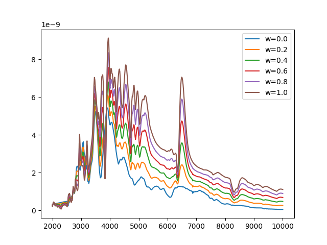
The w=0 spectrum is that of the Ia model, the w=1 spectrum is that of the IIp model, while intermediate spectra are weighted combinations.

We can even fit the model to some data!

model = sncosmo.Model(source=source)
data = sncosmo.load_example_data()
result, fitted_model = sncosmo.fit_lc(data, model,
                                      ['z', 't0', 'amplitude', 'w'],
                                      bounds={'z': (0.2, 1.0),
                                              'w': (0.0, 1.0)})

sncosmo.plot_lc(data, model=fitted_model, errors=result.errors)

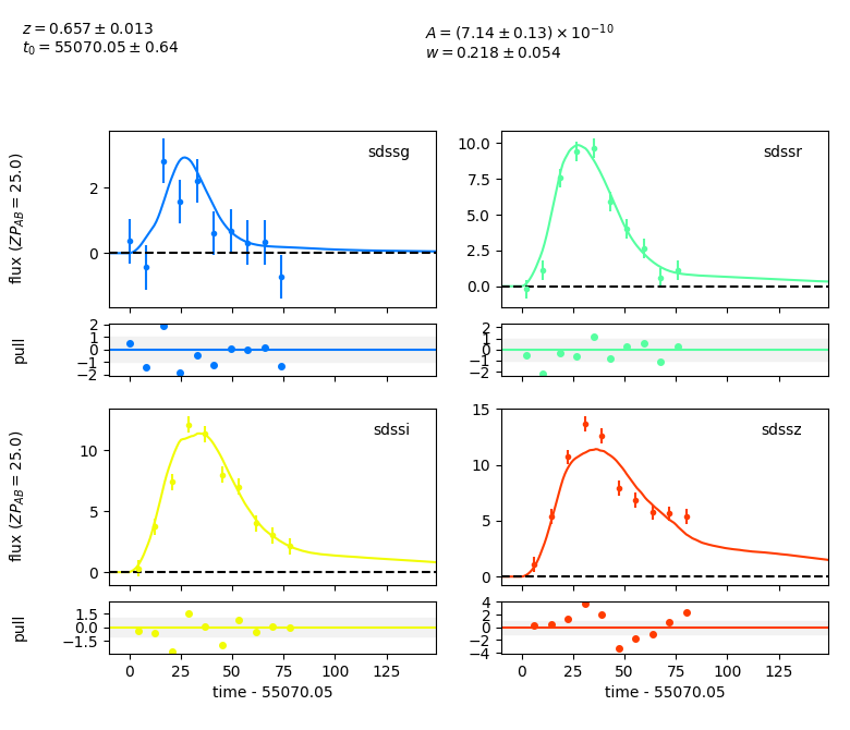
<Figure size 780x670 with 8 Axes>

The fact that the fitted value of w is closer to 0 than 1 indicates that the light curve looks more like the Ia template than the IIp template. This is generally what we expected since the example data here was generated from a Ia template (although not the Nugent template!).